When talking about the most popular method of performing more advanced lookups, INDEX and MATCH easily comes to mind. And for good reason — INDEX and MATCH is convenient and flexible, allowing you to perform both vertical and horizontal lookups, as well as case-sensitive, left, 2-way, and even lookups based on several criteria. If you’re looking to improve your skills in using Excel, INDEX and MATCH should be part of your list.
In this article, we’ll explain in simple terms how to use INDEX and MATCH together to perform lookups. We’ll talk about INDEX first, MATCH, then finally we’ll combine these two. Let’s start!
The INDEX Function
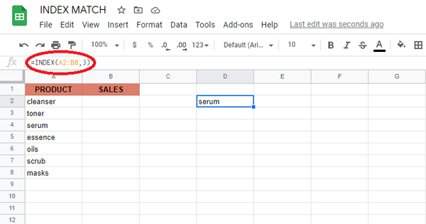
Excel’s INDEX function is incredibly efficient and powerful, often used in a wide range of Excel formulas, particularly advanced formulas. But how does it work? To put it simply, INDEX functions by retrieving the value at a specific location in a range. In the example below, let’s say you want to get the name of the 3rd product (serum) using a formula.
Use INDEX: =INDEX(A2:B8,3)
Suppose you want to get the sales for serums with INDEX? Simply provide both a row number and a column number, and provide a larger range. The INDEX formula below uses the full range of data in A2:B8, with a row number of 3 and column number of 2.
Use INDEX: =INDEX(A2:B8,3,2)

In summary, INDEX gets a value at a given location in a range of cells centered on a numeric position. If the range is one-dimensional, you just need to supply a row number. If the range is two-dimensional, you would need to supply both the row and the column number.
At this point, you might be wondering, “So what? How often do you actually know the position of something in a spreadsheet?”
Exactly. We need a way to find the location of the items we’re searching for.
This is where MATCH comes in
The MATCH Function
The sole purpose of the MATCH function is to identify an item’s position in a range. Take the example below — we can use MATCH to get the position of the planet Mars in this list of planets.
USE MATCH: =MATCH(“mars”,A2:A9,0)

Match returns 4, since “Mars” is the fourth item on the list. Take note that MATCH is not case-sensitive.
Important: The last argument in the MATCH function is what’s called a match type. Match type is critical and controls whether the matching is exact or approximate. In certain instances, you want to use zero (0) to compel the same match action. Match type defaults to 1, which implies an approximate match, so it’s necessary to set a value.
Combining INDEX and MATCH
Now that we know how to use each function, we now move on to combining both in one formula. Take a look at the data below, a table showing a list of flowers and their corresponding sales numbers for three months: October, November, December.

Let’s say we want to write a formula that returns the sales number for February for a given salesperson. Based on the discussion about INDEX, we already know that we can put a row and column number to find a value. So if we want to know the November sales number for the flower Rose, we provide the range B2:D9 with a row 6 and column 2.
Use INDEX: =INDEX(B2:D9,6,2) // returns 7444

In short:
INDEX needs numeric positions.
MATCH finds those positions.
What about VLOOKUP?
After all this, you might be asking why we even bother to use INDEX MATCH. Isn’t VLOOKUP just as good?
Not exactly. Here are a few reasons you might want to use INDEX MATCH instead:
- You don’t need to count. With INDEX MATCH, there is no more question about counting to find out which column you need to pull out of. Just pick the search column and the results column, and you’re done.
- You can insert columns safely. With VLOOKUP, if you insert a column between the start of your table and the column you wish to link, the formula would break—the column index number inside your VLOOKUP will not be modified. INDEX MATCH, on the other hand, securely updates no matter where you insert columns.
- You can lookup backwards. VLOOKUP merely allows you to look up from the columns in front of your starting point. Not so for INDEX MATCH—you can pull out whatever column you like.
- Separate formulas. You don’t need to recall different formulas for VLOOKUP and HLOOKUP.
- More complex functionality. INDEX MATCH does not end with the tutorial above. You may also use the INDEX MATCH MATCH to search through rows and columns, or use the INDEX MATCH for different parameters.
Now you know how to use INDEX MATCH!